Basics of Neural Networks
What is a Neuron?
A Neuron takes input, does some math with them, and produces an output.
Image representation for a 2-input neuron is:
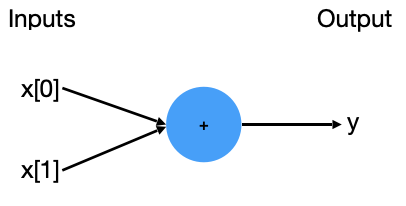
Mathematically
Given the input features x[0], x[1], the output label is computed from left to right. There are 3 computations happening here:
- The inputs are multiplied by weights w[0], w[1]:
\[
x[0]*w[0]
\]
\[
x[1]*w[1]
\]
- All the weighted inputs are then added together with a bias b:
\[
(x[0] * w[0]) + (x[1] * w[1]) + b
\]
- At last, the sum is passed through an activation function f:
\[
y=f(x[0] * w[0] + x[1] * w[1] + b)
\]
Programmatically
| neuron.py |
|---|
| import numpy as np
def get_inputs() -> list[int]:
# Return 2 random inputs
return [12, 24]
def get_weights() -> list[int]:
# Return 2 random weights
return [19, 23]
def get_bias() -> int:
# Return 1 random bias
return 7
def activation_function_sigmoid(x) -> float:
# Our activation function: f(x) = 1 / (1 + e^(-x))
return 1 / (1 + np.exp(-x))
class Neuron:
def __init__(self, weights, bias):
self.weights = weights
self.bias = bias
def feedforward(self, inputs) -> float:
# 1. weight inputs
# 2. add bias
# 3. then use the activation function
total = np.dot(self.weights, inputs) + self.bias
return activation_function_sigmoid(total)
inputs = get_inputs()
weights = get_weights()
bias = get_bias()
neuron = Neuron(weights, bias)
output = neuron.feedforward(inputs)
print(output)
|
What is a Neural Network?
A Neural Network is a bunch of Neurons connected together.
A NN is trained on an input-dataset, during the training it's weights and biases are learned, from which we can predict the output with "high" accuracy. Here, accuracy of correct output/prediction depends only on how well the NN is trained.
Image representation for a 4-input Neuron Network, with 1 hidden layer is:
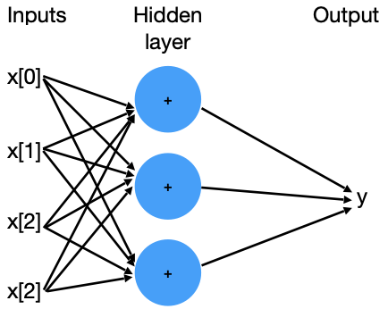
Mathematically
Given the input features x[0], x[1], x[2], x[3], and 3 hidden neurons h[0], h[1], h[2], the output label is computed from left to right. There are 3 computations happening here:
- The inputs are multiplied by weights w[0,0], w[0,1], w[0,2], w[0,3] for hidden neuron h[0] would be:
\[
x[0]*w[0,0]
\]
\[
x[1]*w[0,1]
\]
\[
x[2]*w[0,2]
\]
\[
x[3]*w[0,3]
\]
- All the weighted inputs are then added together with a bias b[0], for hidden neuron h[0], with an activation function f:
\[
h[0] = f(x[0] * w[0,0] + x[1] * w[0,1] + x[2] * w[0,2] + x[3] * w[0,3] + b[0])
\]
- Similarly, for hidden neurons h[1], h[2], and their bias b[1], b[2]:
\[
h[1] = f(x[0] * w[1,0] + x[1] * w[1,1] + x[2] * w[1,2] + x[3] * w[1,3] + b[1])
\]
\[
h[2] = f(x[0] * w[2,0] + x[1] * w[2,1] + x[2] * w[2,2] + x[3] * w[2,3] + b[2])
\]
-
Note: Here w[0,0], w[0,1], w[0,2], w[0,3], ... are the weights between the inputs x and the hidden layer h
-
At last, the sum is passed through an activation function f:
\[
y=f(v[0]h[0] * v[1]h[1] + v[2]h[2] + b)
\]
- Note: Here v[0], v[1], v[2] are the weights between the hidden layer h and the output y
Programmatically
| neural_network.py |
|---|
| import numpy as np
def get_inputs() -> list[int]:
# Return 4 random inputs
return [12, 24, 9, 16]
def get_w_weights() -> list[list[int]]:
# Return 3 x 4 matrix of random weights
return [
[19, 23, 14, 2],
[4, 7, 11, 18],
[3, 13, 52, 20],
]
def get_b_biases() -> list[int]:
# Return 3 random bias
return [4, 6, 9]
def get_v_weights() -> list[list[int]]:
# Return 3 random weights
return [5, 10, 15]
def get_b_bias() -> int:
# Return 1 random bias
return 7
def activation_function_sigmoid(x) -> float:
# Our activation function: f(x) = 1 / (1 + e^(-x))
return 1 / (1 + np.exp(-x))
class Neuron:
def __init__(self, weights, bias):
self.weights = weights
self.bias = bias
def feedforward(self, inputs) -> float:
# 1. weight inputs
# 2. add bias
# 3. then use the activation function
total = np.dot(self.weights, inputs) + self.bias
return activation_function_sigmoid(total)
class NeuralNetwork:
def __init__(self, w_weights, b_biases, v_weights, bias):
self.h1 = Neuron(w_weights[0], b_biases[0])
self.h2 = Neuron(w_weights[1], b_biases[1])
self.h3 = Neuron(w_weights[2], b_biases[2])
self.y = Neuron(v_weights, bias)
def feedforward(self, inputs) -> float:
# For all hidden neurons, run the feedforward method
out_h1 = self.h1.feedforward(inputs)
out_h2 = self.h2.feedforward(inputs)
out_h3 = self.h3.feedforward(inputs)
# The inputs for y are the outputs from h1, h2 and h3
out_y = self.y.feedforward([out_h1, out_h2, out_h3])
return out_y
inputs = get_inputs()
w_weights = get_w_weights()
b_biases = get_b_biases()
v_weights = get_v_weights()
b_bias = get_b_bias()
neural_network = NeuralNetwork(w_weights, b_biases, v_weights, b_bias)
output = neural_network.feedforward(inputs)
print(output)
|
> python3 neural_network.py
1.0
What is a Loss Function?
Loss Function (along with activations) are responsible for fitting the given training data in the model.
When the model generate predictions, we compute a loss by comparing these predictions to the actual (target) values. Based on the value of Loss Function, the weights are updated.
Loss function (also known as cost function OR error function), seeks to minimise the error, hence the output is simply called loss.
Let's take an example of Mean Squared Error Loss (MSE), is the average/mean of squared differences between the actual-value and predicted-value.
Mathematically
\[
MSE = 1 / n \sum_{i=1}^{n}(Y_i - \hat{Y_i})^2
\]
Where,
- n is the number of samples/predictions.
- \(Y_i\) is a vector of actual (target) values.
- \(\hat{Y_i}\) is a vector of predicted values.
Programmatically
| mean_squared_error_loss.py |
|---|
| import numpy as np
def get_targets() -> list[int]:
# Return 3 random targets
return [4, 9, 6]
def get_predictions() -> list[int]:
# Return 3 random predictions
return [4, 8, 6]
def mean_squared_error(targets, predictions) -> float:
# Our Loss/Cost function: Mean Squared Error (MSE)
difference = np.subtract(targets, predictions)
squared_difference = difference**2
mean_squared_difference = np.mean(squared_difference)
return mean_squared_difference
target_values = get_targets()
predicted_values = get_predictions()
mse_loss = mean_squared_error(target_values, predicted_values)
print(mse_loss)
|
> python3 mean_squared_error_loss.py
0.3333333333333333
What is Activation Function?
Activation function is a function, which when applied to a neuron/cell output, updates/activates/de-activates the output value. The resulting output value can be used as our final output, or can be fed into another neuron as it's input.
Let's take an example of an activation function which outputs value only between the range 0 and 1, called Sigmoid activation function (also known as Logistic activation function).
Mathematically
\[
S(x) = \frac {1} {1+e^{-x}}
\]
Where,
- \(x\) is the input to the Sigmoid activation function.
- \(e \approx 2.71\) is the base of the natural logarithm
Programmatically
| sigmoid_activation_function.py |
|---|
| import math
import numpy as np
def get_neuron_output() -> list[int]:
# Return 1 random integer
return 126
def sigmoid_activation_function(x) -> float:
# Our Sigmoid activation function: 1 / ( 1 + e^{-x} )
return 1 / (1 + math.exp(-x))
neuron_output = get_neuron_output()
sigmoid_output = sigmoid_activation_function(neuron_output)
print(sigmoid_output)
|
> python3 sigmoid_activation_function.py
1.0